Last post we compared our distributed engine performance against Apache Spark. This sparked some interest; “How does it perform against single node Polars”. That interest is shared by us. Polars has gotten popularity by massively increasing single node performance and by reducing complexity by delaying the need for Spark and distributed compute (with the release of distributed Polars we postpone the need indefinitely). Some voices in the industry claim that if you can process data single node, this is always faster and cheaper, today we learn a bit more nuance story… It depends. This post we’ll see when you can expect distributed Polars to beat single node and vice versa.
1. Distributed engine
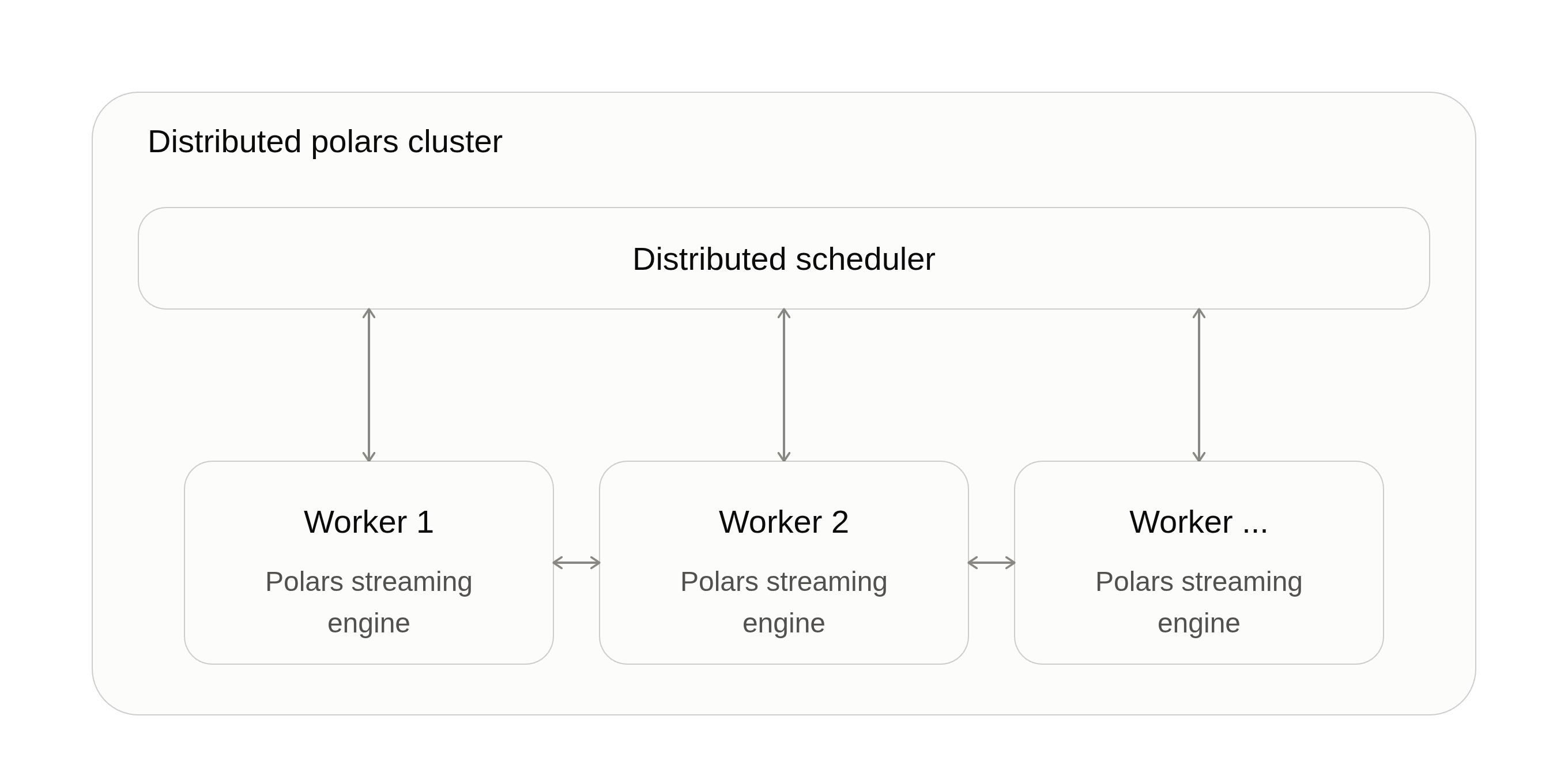
The distributed engine uses our open source streaming engine for performance, but adds a distributed planner and communication layer on top of it. Any change we make in our open source streaming engine therefore immediately translates to improvements in the distributed engine as well, plus this guarantees that the engine semantics (e.g. nulls handling) remain the same. This aligns the interests of our open source and distributed offering.
There are differences in performance characterstics between the two which we can see in the results below.
2. Setup
Polars Decision Support (PDS-H) is an open implementation derived from the TPC-H benchmark. It uses the TPC-H data model, data generation methodology, and query workload to measure analytical query performance across a potential range of dataset sizes1.
The benchmarks were run on a scale factor of 1000, which means the dataset used is the size of roughly a terabyte of data if it were stored in uncompressed CSV with the data coming directly from AWS S3, including network I/O for reading. Both machines are priced similar on AWS. To avoid any outliers (e.g. bad network connections), we ran the benchmarks three times and measured the fastest result. The code can be found in the following GitHub repository.
2.1 Hardware specifications
Comparing distributed compute to single node isn’t an apples to apples comparison, for this reason we tried to stay within the same family and ensure we have the same vCPU, RAM and storage between the two.
- Single node: m8i.32xlarge (128 vCPUs, 512 GB RAM)
- Distributed: 32 * m8i.xlarge (4 vCPUs, 16 GB RAM)
3. Results
Below are the per-query results comparing single node Polars against distributed Polars. For most queries the two run close to eachother, but on some queries single node wins while on others distributed wins.
Overall this leads to the following summary with the distributed engine being slightly faster than single node overall:
This results goes against the conventional wisdom that if it fits on a single machine it should be faster due to the lack off data shuffling. We can see this for heavy join queries (Q8 & Q9) single node is much faster than distributed as a lot of time is spent shuffling data over the network.
3.1 Network I/O
For queries Q6, Q14, Q15 distributed is a lot faster than single node. The main reason for this, is that those queries are I/O-bound. For AWS, network speeds do not scale linearly with the number of vCPUs, but work on a credit system. This system favors many small machines over large ones. If we look at Q6 in the benchmark:
q = (
    lineitem.filter(
        pl.col("l_shipdate").is_between(
            date(1994, 1, 1), date(1995, 1, 1), closed="left"
        )
    )
    .filter(pl.col("l_discount").is_between(0.05, 0.07))
    .filter(pl.col("l_quantity") < 24)
    .with_columns(
        (pl.col("l_extendedprice") * pl.col("l_discount")).alias("revenue")
    )
    .select(pl.sum("revenue"))
)
This query exists almost purely of network I/O, reading in the lineitem table (6B rows) with some predicate filtering and then aggregating the results. The bottleneck here is the speed at which the data is being read from S3, not the CPU or memory.
If we compare the network bandwidth available for each setup:
| Setup | Per-instance baseline | Per-instance burst | Instances | Aggregate baseline | Aggregate burst |
|---|---|---|---|---|---|
Single node (m8i.32xlarge) | 50 Gbps | 50 Gbps (sustained) | 1 | 50 Gbps | 50 Gbps |
Distributed (m8i.xlarge) | 1.88 Gbps | 12.5 Gbps | 32 | 60.16 Gbps | 400 Gbps |
The m8i.32xlarge runs at a sustained 50 Gbps and does not burst. The smaller m8i.xlarge has a lower baseline of 1.88 Gbps but can burst up to 12.5 Gbps on network I/O credits. Spread over 32 workers, the cluster’s aggregate baseline (~60 Gbps) already exceeds the single node, and its aggregate burst reaches 400 Gbps, 8x the single node, which is why we see such a large difference in performance for Q6. For a fresh machine you get roughly an hour of full burst capacity before it starts to throttle back to the sustained baseline2.
In queries Q8, Q9, we see that single node is much faster. The reason for this is that these queries have many joins, which in turn lead to many shuffles. Even though you have more I/O capacity in the cluster, increasing the total I/Os needed by the extra shuffles is detrimental and single node wins.
We are planning to include bloom filters pushdown between stages. This will drastically reduce the amount shuffled between stages and might change this verdict in the future.
3.2 Numa awareness
In essence, this comes down to a choice between scaling vertically or horizontally. In both directions we can get the same vCPU and RAM, however we saw that I/O doesn’t scale linearly. vCPU does scale linearly, but not all vCPU count is created equal. If you increase the amount of vCPU’s on a single machine, at one point CPU cores are assigned to different NUMA (non uniform memory access) regions. Between these regions, reading memory is much more expensive and can become a bottleneck.
Our streaming engine has a concept of work stealing built into it. This means that when a thread is idle, it can steal work from other cores to increase performance. This works well for smaller machines (with single NUMA regions), but on large machines a CPU is typically divided over multiple different physical (NUMA) nodes, in which case work stealing can lead to performance degradation due to data transfer.
Our test setup m8i.32xlarge is divided over two NUMA nodes each with their own memory. Our streaming engine is currently stealing work across NUMA nodes, which leads to memory contention and overall slower performance.
We are in working on solving this issue and have run a secondary benchmark on a smaller single node (r8i.16xlarge) with a single NUMA node. The results show that single node execution is faster on most queries, expect for ones with heavy read I/O.
4. Conclusion
The decision to use distributed or single node compute is not only influenced by scale, but it turns out to also be influenced by speed and latency, and therefore cost. Polars will optimize both engines and ensure that we utilize the maximum of the trilemma I/O, CPU and RAM. By running this benchmark we show that choosing your scaling method is a nuanced story. One that we want to make easier. Overall, we recommend using the query profiler for both cases to understand the performance characteristics of your queries.
Appendix: Non-numa benchmark on r8i family
We ran the benchmark again on an r8i.16xlarge instance, which has a single NUMA node. The number of cores drops significantly from 128 to 64, meaning many of the queries now are not network bound, but CPU bound. This lead to the following results:
Footnotes
-
While PDS-H closely follows the TPC-H specification, it is not an officially audited or certified TPC-H benchmark. Consequently, PDS-H results are intended for comparative evaluation within PDS-H and are not directly comparable to published TPC-H benchmark results. ↩
-
For a full guide on AWS network bandwith, you can find the offical documentation here ↩