Polars Cloud and On-Premises now include a query profiler that shows resource usage and per-stage performance metrics, such as CPU/RAM/network utilization, I/O active time, shuffle percentage, and more.
Picking the right instance type and cluster size for a distributed query is usually guesswork. You overprovision and pay too much, or underprovision and wait, and it can be hard to know which resource was the bottleneck.
In this post, we run TPC-H Q21 on a 1 TB dataset, starting from a single large general-purpose instance. Each run, we use profiler insights and query runtime to make one targeted change. Rather than running a grid search across dozens of configurations, you can read the profiler output and know which lever to pull next. Five runs take us from the baseline to an optimal configuration which is 54% faster and 64% cheaper.
Introducing the Query Profiler
The query profiler is a new tool available on Polars Cloud and On-Premises that gives you a look into your query’s performance. It allows you to inspect different aspects of your query. Here is a quick walkthrough of the profiler in action:
Let’s go through each of these screens step by step.
The Logical Plan
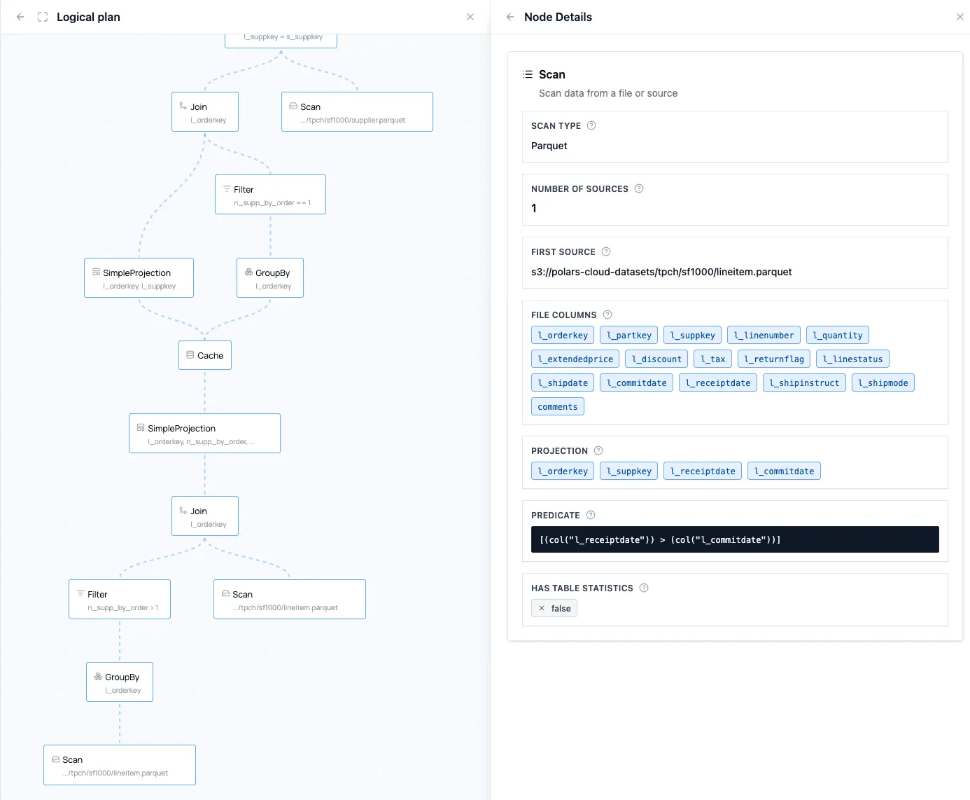
When you send your query to the engine, it gets transformed into a tree of operations that gets optimized. The result is an optimized logical plan, which can be viewed under the Query Details.
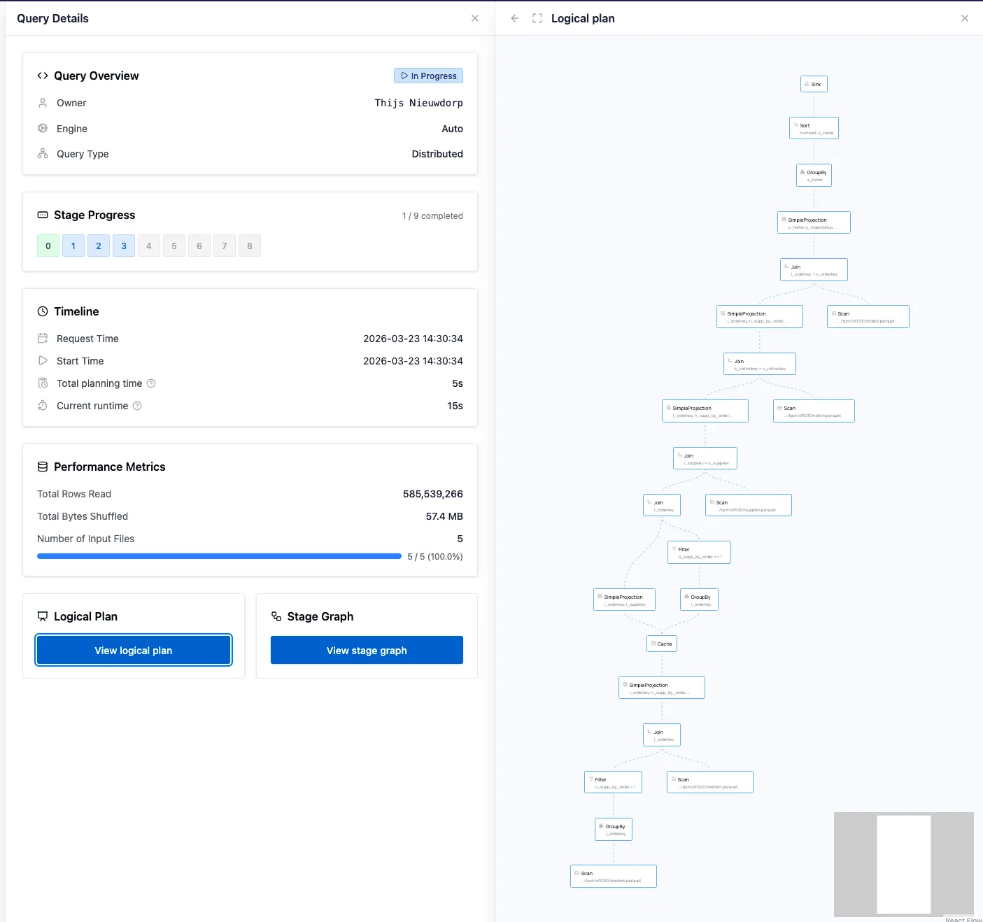
You can click the nodes to find more specific information about the operations and the optimizations (such as predicate or projection pushdown):
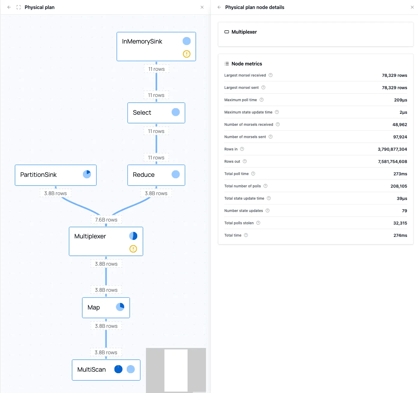
The Physical Plan
The logical plan is sent to the query planner, which transforms the optimized logical plan into a physical plan. The physical plan contains all the necessary information on how the query will be executed. It also shows execution progress in real time. In the details of each node it provides metrics about the amount of data that goes through the node, and the time spent there.
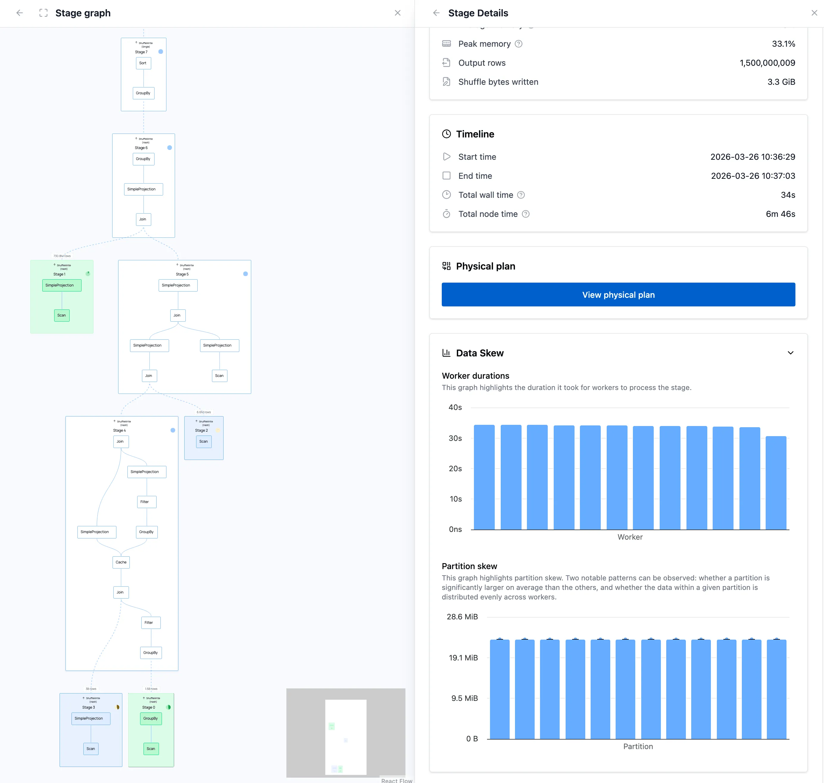
The Stage Graph
For distributed queries, the stage graph shows how work is spread over workers, and how it is split into stages in case data needs to be shuffled.
Resource Usage
On the dashboard overview of your cluster you can see aggregated cluster resource usage, which can help you find resource bottlenecks in your configuration.
And besides that on the Nodes tab you can inspect individual Node resource usage for a more detailed view. Especially on single-node queries, this can help you find bottlenecks. We will use this view in the example later in the blog post.
Indicators
On top of this, indicators on nodes and stages can highlight potentially memory-intensive operators, single-node execution, and other issues that might affect performance.

You can find more information on the query profiler in our User Guide.
Together, these views make it easier to move from “this query runs in x time” to actionable insights such as “this stage is I/O-bound” or “this operation is doing most of the work.” Let’s go through an example of how you could use the query profiler.
Example: Optimizing Cluster Configuration
To showcase the query profiler we’ll go through an example in which we’ll optimize the cluster configuration on which a query runs.
The Query
The query we’re using in our example is query 21 from the TPC-H benchmark. TPC-H is an industry-standard OLAP benchmark consisting of 8 tables and 22 analytical queries (aggregations, multi-table joins, filters) modeled after a wholesale supplier database. The dataset scales via a scale factor (SF), where SF 1 ≈ 1 GB, making it a convenient tool for testing query performance at different data volumes. In this blog we will be running a query from the TPC-H benchmark, query 21, on a scale factor of 1000. Some of the datasets contain up to 6 billion rows, making the total dataset size 1TB uncompressed.
This query identifies suppliers, for a given nation, whose product was part of a multi-supplier order where they were the only supplier who failed to meet the committed delivery date. This involves multiple datasets that are (self-)joined and aggregated, which gives us enough complexity to explore what the query profiler has to offer.
This is the code for the query:
import polars as pl


S3_BASE = "s3://polars-cloud-datasets/tpch/sf1000"

lineitem = pl.scan_parquet(f"{S3_BASE}/lineitem.parquet")  # 171.1 GB
nation   = pl.scan_parquet(f"{S3_BASE}/nation.parquet")    # 3.2 KB
orders   = pl.scan_parquet(f"{S3_BASE}/orders.parquet")    # 40.3 GB
supplier = pl.scan_parquet(f"{S3_BASE}/supplier.parquet")  # 494.1 MB


def tpch_q21(lineitem, nation, orders, supplier):
    """TPC-H Q21: Suppliers Who Kept Orders Waiting"""
    nation_name = "SAUDI ARABIA"

    items = (
        lineitem.group_by("l_orderkey")
        .agg(pl.col("l_suppkey").len().alias("n_supp_by_order"))
        .filter(pl.col("n_supp_by_order") > 1)
        .join(
            lineitem.filter(pl.col("l_receiptdate") > pl.col("l_commitdate")),
            on="l_orderkey",
        )
    )

    return (
        items.group_by("l_orderkey")
        .agg(pl.col("l_suppkey").len().alias("n_supp_by_order"))
        .join(items, on="l_orderkey")
        .join(supplier, left_on="l_suppkey", right_on="s_suppkey")
        .join(nation, left_on="s_nationkey", right_on="n_nationkey")
        .join(orders, left_on="l_orderkey", right_on="o_orderkey")
        .filter(pl.col("n_supp_by_order") == 1)
        .filter(pl.col("n_name") == nation_name)
        .filter(pl.col("o_orderstatus") == "F")
        .group_by("s_name")
        .agg(pl.len().alias("numwait"))
        .sort(by=["numwait", "s_name"], descending=[True, False])
        .head(100)
    )
For each cluster configuration, we run the query three times and take the minimum duration. We then compare those runtimes to find a configuration that is both fast and cheap.
Large Single Instance Run
To run this query on Polars Cloud, we wrap it in a ComputeContext and call .remote(ctx).execute().
The instance_type and cluster_size parameters are the two levers we’ll tune throughout this post.
We will tweak the configuration step-by-step based on metrics such as CPU utilization, RAM utilization, network bandwidth, I/O active time, and shuffle percentage.
Polars Cloud will then take care of executing the query on the requested cluster automatically.
To make inspecting the resource usage for this query simple, we first run the query on a single instance.
For this we pick the m7i.48xlarge, which has 192 vCPUs and 768 GB RAM.
This is the most recent Intel general-purpose instance available in our availability region, and it is comfortably large enough to fit the query.
The Parquet files we scan are compressed on disk, but their in-memory footprint during execution is much larger, so we start with a large baseline instance to remove memory pressure as a confounding factor.
with pc.ComputeContext(
    workspace="my-workspace",
    instance_type="m7i.48xlarge",
    cluster_size=1,
) as ctx:
    result = tpch_q21(lineitem, nation, orders, supplier).remote(ctx).execute()
This query sets the following baseline, which we will try to improve on:
| Cluster configuration | Query runtime | Cost |
|---|---|---|
| m7i.48xlarge x 1 | 157s | $0.470 |
Analyzing the Query
While executing the query, you can see the resource usage in the cluster dashboard. It shows which resources are used the most, and which ones might be underused, which will help us tweak the cluster configuration.
Note: a future version of the query profiler will display resource usage graphs for all runs stacked below each other, making it easier to compare configurations visually.
On this screen you can see a couple of indications that the resources are not optimally used.
- CPU utilization is generally low, but has bursts of 100%. This indicates processing is blocked by other bottlenecks.
- RAM usage never goes above 40%.
- Network I/O seems to block full CPU usage, as the CPU goes to 100% only after the download is done.
Diving deeper into the query, we can view the physical plan.
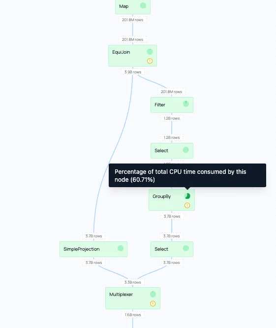
We can see that in the stages taking the most time, the group-by’s take up a lot of time. The physical plan also shows that a lot of time is spent at the scan phase at the start.
Reads and compute happen concurrently in our streaming engine, but slow I/O starves the compute pipeline. Processing catches up faster than data arrives, so the bottleneck is the read throughput. By first focusing on improving the network I/O, we can improve the total runtime of the query.
Scaling Horizontally
In order to only change one variable at a time, we will keep the vCPUs and GB of RAM the same. Instead we will work with multiple smaller instances that have the same total of vCPUs and RAM. The only dial we’ll turn is the cluster size, while simultaneously making the instance size smaller. Because the pricing for this instance family scales proportionally by vCPU, the resulting configurations will have the same price per hour.
We’ll take the same number of vCPUs and RAM, but split it over 12 small machines.
We can do this by using 12 m7i.4xlarge machines, that each have 16 vCPUs and 64GB RAM.
We choose 12 workers because that preserves the baseline exactly: 12 x 16 = 192 vCPUs and 12 x 64 GB = 768 GB RAM.
The price per hour stays the same (m7i.4xlarge costs 1/12 of a m7i.48xlarge, but we’re using 12 of them).
However, we get up to double the bandwidth in total for the same price.
When choosing a number of workers you have to strike a balance: you need enough workers to maximize network bandwidth, but making them too small has its own costs. For this query and dataset, data skew is minimal: intermediate partitions stay small and are distributed evenly across workers. With heavy skew, one worker can end up processing a much larger partition than the others, both slowing down that stage and risking an OOM if the partition exceeds the worker’s available memory. The right cluster size always depends on your specific query and data.
On top of that, small EC2 instances (≤16 vCPUs) have a network bandwidth burst capability funded by credits. They launch with full credits, spend them when exceeding baseline, and earn them back when below it. Burst lasts 5–60 minutes and is best-effort even when credits are available. For our short running query, this is a good match.
Let’s run a query on this new distributed configuration:
ctx = pc.ComputeContext(
    workspace="my-workspace",
    instance_type="m7i.4xlarge",
    cluster_size=12,
)| Cluster configuration | Query runtime | Cost |
|---|---|---|
| m7i.48xlarge x 1 | 157s | $0.470 |
| m7i.4xlarge x 12 | 98s | $0.294 |
The runtime, and with that the cost, is reduced by 37.5% compared to the baseline.
Now that the query runs in distributed mode, we also get a stage graph that shows how work flows through the cluster and when stages complete.
In this run, the stage graph confirms that the query is split into a handful of stages, while the shuffle metrics below show that the exchange between workers is not the dominant cost.
Since we’ve gone distributed, the resource usage becomes a bit harder to track, because we’ve now got 12 nodes that are hard to individually inspect. On top of that we’ve introduced a new aspect to the runtime, data shuffling: operations like joins and aggregations require all rows with the same key to be on the same worker, so each worker re-partitions its data by key and ships those partitions to the responsible workers over the network. We can see the performance metrics about shuffling on the query details, when clicking the query in the cluster dashboard:
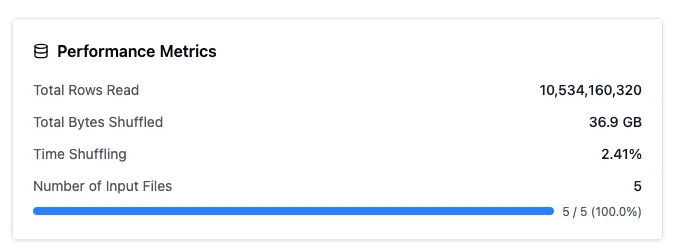
Luckily the time spent shuffling is low, so this is not something we will have to tune further.
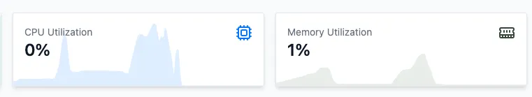
Aggregated cluster resource usage can be seen at the top of the cluster dashboard. Note that the numbers represent current resource usage, while the screenshot was taken after the query completed. The graphs reflect the resource usage during the query.

One thing that still jumps out is the low RAM utilization.
Optimized Instance Type
We can change the instance type of our cluster configuration to a compute optimized instance. Because we don’t use the RAM, a compute optimized instance can give us the same amount of vCPUs, but half the RAM, for a reduced price: 14.8% cheaper. All other specs remain the same.
To make sure our runtime doesn’t go up, we’ll test that configuration.
ctx = pc.ComputeContext(
    workspace="my-workspace",
    instance_type="c7i.4xlarge",
    cluster_size=12,
)| Cluster configuration | Query runtime | Cost |
|---|---|---|
| m7i.48xlarge x 1 | 157s | $0.470 |
| m7i.4xlarge x 12 | 98s | $0.294 |
| c7i.4xlarge x 12 | 91s | $0.232 |
The run was slightly faster and with the reduced rate for a compute optimized instance, that results in a 21.0% reduction in cost compared to the previous step.
During query execution, the peak of memory usage still doesn’t reach above 50%, showing the query can safely run with less RAM. The compute-optimized family is already the lowest RAM-to-vCPU ratio available on AWS, there is no instance type with even less memory at the same core count. Because there are still parts of the query that are CPU bound (100% load), we can’t reduce the number of vCPUs, so this is the smallest instance that can efficiently run the workload.
So far we’ve executed everything on Intel machines. However, AWS also offers their own Graviton CPUs, which they position as having better price-performance.
Moving from Intel to Graviton
Graviton instances offer the same number of vCPUs and RAM as we’ve been using, but are 19% cheaper per hour compared to their Intel alternative. However, hourly rate isn’t everything, and we should still test our runtime on this different CPU architecture:
ctx = pc.ComputeContext(
    workspace="my-workspace",
    instance_type="c7g.4xlarge",
    cluster_size=12,
)| Cluster configuration | Query runtime | Cost |
|---|---|---|
| m7i.48xlarge x 1 | 157s | $0.470 |
| m7i.4xlarge x 12 | 98s | $0.294 |
| c7i.4xlarge x 12 | 91s | $0.232 |
| c7g.4xlarge x 12 | 84s | $0.173 |
A combination of improvement in runtime together with lower hourly rates results in a 25% cost improvement compared to the previous step.
As a final optimization, there is also a newer Graviton generation available.
Latest Generation Instances
Our initial machine used an Intel architecture and in our availability region these were only available in 7th gen machines. For our final optimization we will resort to the latest available generation of these machines in our availability region, generation 8. Although these machines are 10% more expensive per hour compared to the 7th gen, they might run the workload faster. According to AWS, C8g instances offer up to 30% better performance than the seventh-generation AWS Graviton3-based C7g instances. Let’s see if they bring a runtime improvement that will lead to a lower total cost.
ctx = pc.ComputeContext(
    workspace="my-workspace",
    instance_type="c8g.4xlarge",
    cluster_size=12,
)| Cluster configuration | Query runtime | Cost |
|---|---|---|
| m7i.48xlarge x 1 | 157s | $0.470 |
| m7i.4xlarge x 12 | 98s | $0.294 |
| c7i.4xlarge x 12 | 91s | $0.232 |
| c7g.4xlarge x 12 | 84s | $0.173 |
| c8g.4xlarge x 12 | 73s | $0.166 |
This final step is a smaller incremental win than the earlier changes, but it still makes the query 13.1% faster and 4.0% cheaper compared to the previous c7g setup.
That concludes our optimization. Let’s summarize what we walked through.
Conclusion
The new query profiler removes guesswork from how your query is performing. On top of that, Polars Cloud makes it easy to quickly change your query’s infrastructure. Rather than running a grid search across dozens of configurations, the profiler guides infra decisions. Five runs took us from a $0.470 single-node baseline to a $0.166 optimal configuration: 54% faster and 64% cheaper.
In practice, the workflow is straightforward:
- Low CPU usage together with high download bandwidth points to an I/O-bound query, so scaling out can help.
- Low memory utilization suggests you may be able to move to a compute-optimized instance family and lower cost.
- Low shuffle percentage in a distributed run suggests that the cluster is not spending most of its time exchanging data between workers.
Get started on https://cloud.pola.rs/