
Query profiles are a great way to understand what Polars is doing during execution, but up until now only the people in your workspace could see them. When a query didn’t perform as expected and you wanted someone else to have a look (a colleague in another team, or us), you had to fall back to screenshots or copy pasting the query plan. With this release you can share the query profile itself by sending a link. In this post we’ll show how to share a query and walk through an example profile of one of the TPC-H queries, which you can open here.
Sharing a query
Sharing is done from the Queries tab in Nanook. Select the query you want to share, click share and choose how long the link should be valid (one week up to no expiry). You can revoke the link at any time.
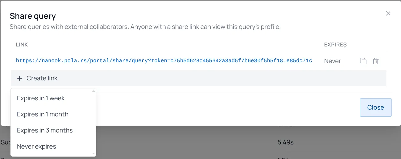
Whoever opens the link doesn’t need an account. They only get to see this one query profile: the plan, the stages and the metrics. They don’t get access to your workspace, your other queries or your data.
Example Query to profile
To show what a shared profile looks like we ran query 17 of the TPC-H benchmark on a scale factor of 1000 (roughly 1TB of data) on a cluster of 32 machines. The query answers the following question: how much yearly revenue would be lost if we no longer took small orders for a specific type of part? Small here means less than 20% of the average quantity ordered for that part.
import polars as pl
import polars_nanook as pn

# TPC-H data generated at scale factor 1000, stored as parquet
BASE = "s3://<your-bucket>/tpch/sf1000"

ctx = pn.ComputeContext(instance_type="m8i.xlarge", cluster_size=32)

part = pl.scan_parquet(f"{BASE}/part/*.parquet")
lineitem = pl.scan_parquet(f"{BASE}/lineitem/*.parquet")

q1 = (
    part.filter(
        pl.col("p_brand") == "Brand#23",
        pl.col("p_container") == "MED BOX",
    )
    .join(lineitem, how="left", left_on="p_partkey", right_on="l_partkey")
)
query = (
    q1.group_by("p_partkey")
    .agg((0.2 * pl.col("l_quantity").mean()).alias("avg_quantity"))
    .join(q1, on="p_partkey")
    .filter(pl.col("l_quantity") < pl.col("avg_quantity"))
    .select((pl.col("l_extendedprice").sum() / 7.0).round(2).alias("avg_yearly"))
)

query.remote(ctx).distributed().execute()
import polars as pl
import polars_nanook as pn
# TPC-H data generated at scale factor 1000, stored as parquet
BASE = "s3://<your-bucket>/tpch/sf1000"
ctx = pn.ComputeContext(instance_type="m8i.xlarge", cluster_size=32)
query = pl.sql(
f"""
SELECT
ROUND(SUM(l_extendedprice) / 7.0, 2) AS avg_yearly
FROM read_parquet('{BASE}/lineitem/*.parquet') AS lineitem
JOIN read_parquet('{BASE}/part/*.parquet') AS part
ON p_partkey = l_partkey
WHERE p_brand = 'Brand#23'
AND p_container = 'MED BOX'
AND l_quantity < (
SELECT 0.2 * AVG(l_quantity)
FROM read_parquet('{BASE}/lineitem/*.parquet')
WHERE l_partkey = p_partkey
)
"""
)
query.remote(ctx).distributed().execute()The profile
You can open the profile here and follow along.
When you open the profile you land on the query details. At the top you find the duration and the progress of each stage, at the bottom the performance metrics: how many rows and bytes were read and how much data was shuffled between machines. In between are two views of the query. The logical plan shows your query after our optimization: what Polars is going to compute, which columns it reads and where the filters are applied. The stage graph shows how that plan runs on the cluster. The query is split into stages that run on workers, and the lines between them are shuffles, where data is sent between machines, labelled with the number of rows that go over them. Clicking a node in either view shows its details.
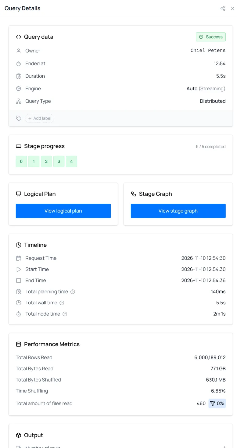
The query ran in 5.5 seconds, of which 140ms was spent on planning. The 32 workers read 460 files containing 6 billion rows (77.1 GB) and ran the query in 5 stages. The sum of all wall time of the workers equals 2 minutes and 1 second, the Total node time compared to the actual wall time of 5 seconds. Only 630 MB was shuffled between workers, and shuffling took 6.65% of the time. For a query that reads 77 GB that is very little. Two optimizations make this possible: a bloom filter that throws away most of the data before it is shuffled, and computing the join of the parts and order lines only once. Let’s look at both.
Bloom filter
When you join two tables on a cluster, the rows with the same key have to end up on the same machine. This means sending data over the network (a shuffle), which is one of the most expensive things a distributed engine does. A bloom filter can reduce the amount of data shuffled if we expect to filter / match the data in a later stage (e.g. with a join). You can think of it as a small summary of a list of keys. Ask it whether a key is in the list and it answers either “maybe” or “definitely not”.
In our query the order lines table is by far the largest with 6 billion rows (most of the 77.1 GB under Total Bytes Read). However we later join it with the parts table and only keep any smaller subset of the line item table. Polars builds a bloom filter on the join key, broadcasts it to all workers and filters out rows that are definitely not in the parts table.
You can see this in the stage graph. Stage 0 reads the parts and sends the 199.3K matching keys to every machine in stage 1 (the line marked Broadcast). There, the Filter node next to the Scan of the order lines uses the bloom filter to drop the order lines we don’t need. Only 66.1M of the 6 billion rows leave stage 1, and under Total Bytes Shuffled in the query details you can see that just 630 MB was sent between machines.
Computing the join once
The query uses q1, the matching parts joined with their order lines, twice: once to calculate the average quantity per part and once to compare every order line against that average. Polars rewrites this into a group by and a second join, and computes q1 only once. In the stage graph you can see a Cache node in stage 2: the result of the first join feeds both the GroupBy and the input for the second join. The same happens in stage 0, where the parts are scanned once and used for both the broadcast and the hash shuffle.
The second join doesn’t send its input over the network either. After the first join the order lines are already split across the machines by part key, which is exactly what the second join needs. That’s why the ShuffleWrite on that side is marked Local: the data stays on the machine it’s on, and only the averages from the group by are shuffled.
Up next
We are already working on the next step: connecting your agents to the query profiler through an MCP server, so they can analyze a profile and recommend optimizations.
Try it out!
Go to nanook.pola.rs and run your first query in minutes. If you are an open source Polars user, add pl.Config.enable_monitoring() to profile your local queries in the same interface.
Let us know what you think on our Discord or add feature requests to our issue tracker.