This post is written by Thijs Nieuwdorp and Tom Drabas.
-
Thijs Nieuwdorp is a Data Scientist at Xomnia and a co-author of Python Polars: the Definitive Guide.
-
Tom Drabas is Senior Developer Relationship Manager at NVIDIA.
Improving the Polars GPU engine
One of the core philosophies of Polars is to utilize all available cores on your machine. One type of computation core that makes up a lot of the compute power is in Graphics Processing Units, or GPU. Polars, which was already known for its high performance, has pushed its limits through a collaboration with NVIDIA, unlocking even more power by integrating a GPU engine that promises to accelerate compute-bound queries. At its core it leverages NVIDIA cuDF, a DataFrame library that is built on the CUDA platform, to offload intensive operations such as group bys, joins and string manipulation onto the parallel architecture of modern NVIDIA GPUs. With virtually zero code changes, users can trigger GPU execution, simply by specifying the GPU engine using the following parameter: .collect(engine=”gpu”). In case the operation isn’t compatible it falls back gracefully to normal CPU execution, guaranteeing a result.
Normally, the GPU engine runs calculations by loading data onto Video Random-Access Memory (VRAM), the working memory of the GPU. This has a lightning fast connection to the computation cores of the GPU. Unfortunately, GPUs generally tend to have less VRAM available compared to system RAM. This limits the capabilities of the GPU engine when working with large datasets. The RAPIDS team is constantly working on new features that alleviate this problem. One of their recently implemented techniques is the introduction of CUDA’s Unified Virtual Memory (UVM).
But, does UVM allow for larger-than-VRAM operations? And does it bring any performance overhead? Let’s find out.
Larger-Than-VRAM
Unified Virtual Memory combines the system’s RAM (also called host memory) with the VRAM (also called device memory) of the GPU. This allows the GPU engine to work with a memory pool that’s larger than just the VRAM, preventing out-of-memory errors. To understand how this feature works, you will first need to dive into how memory works in general. For this you need to know a few key terms:
Every object that exists in memory has an assigned memory address. The memory address space is divided into pages, or page files, that are contiguous chunks of memory of a set size. The address space can be bigger than RAM, in which case for example a page can reside on secondary storage in order to allow the aggregate size of the address spaces to exceed the physical memory of the system. In the case of UVM, this secondary storage is the RAM. The technique of storing pages on and retrieving them from secondary storage is called swapping.
When an application tries to access an address that’s not currently mapped to VRAM, a page fault occurs. To handle this fault, the GPU has a Page Migration Engine that will handle swapping the right page into VRAM. What follows below is a gross oversimplification of what that would look like under the hood.
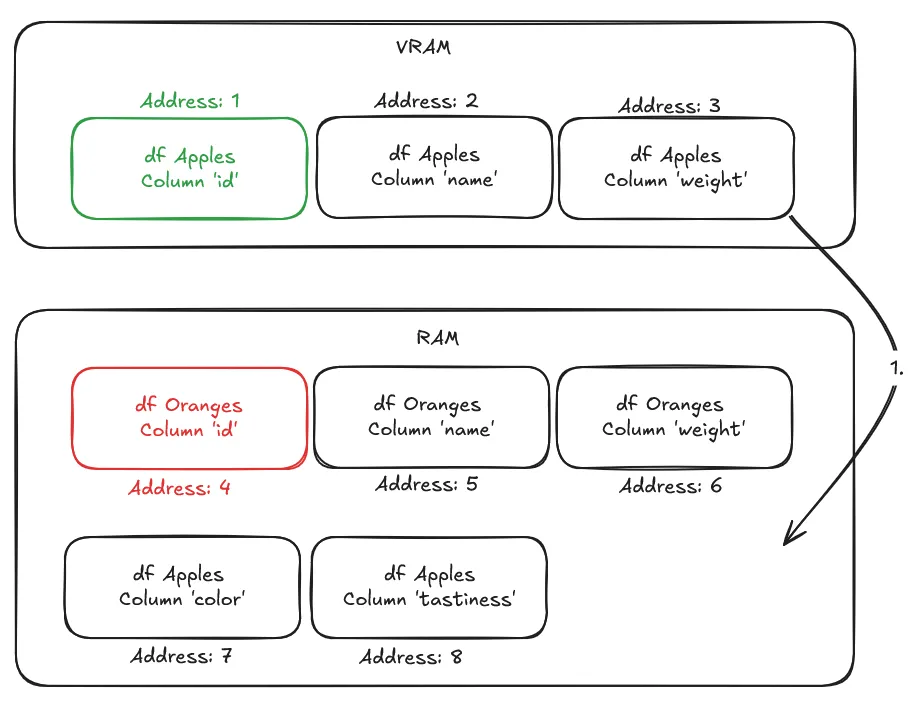
Say we want to join Oranges to Apples on their respective id columns, to compare the two datasets. However, we just did an analysis on the apples’ names and weights, which means that only Apples data is currently loaded in VRAM.
To execute the join, the application requests “Address 4” which contains data from the oranges’ id column. However, this column currently resides in RAM, causing a page fault. To swap it into VRAM the Migration Engine will do the following:
- Free VRAM by swapping least-recently-used pages from VRAM to RAM.
- Map the newly freed VRAM to “Address 4”, which the application was trying to access.
- Swap into VRAM, from RAM, the page that is supposed to be at that address, and contains the column “id”.
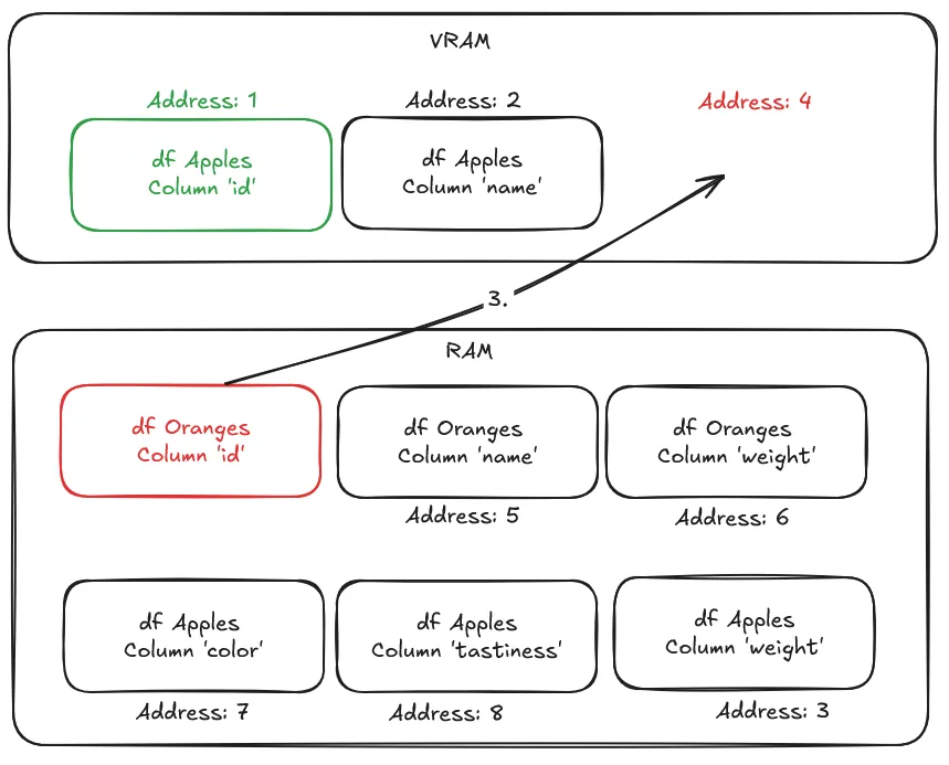
- Retry accessing the memory address and resume the program where it left off. This time, it successfully retrieves the data.
While this swap happens, the program is paused, and thus incurs a performance penalty whenever a page fault occurs. The NVIDIA driver employs heuristics to maintain data locality, the practice of storing data near the processing unit that will consume it, reducing data movement and latency in data-intensive applications. This prevents excessive page faults. On top of these heuristics you can use the CUDA API to prefetch specific objects to VRAM to prevent page faults from happening. In this case, the Polars CUDA-accelerated engine tells the CUDA API to prefetch data based on the type of queries that are being executed to minimize page faults.
All of these techniques allow GPU calculations on “larger-than-VRAM” dataset, possibly at the cost of some performance, due to page migrations. To help you pick the best configuration for your use case, let’s find out more about the perks and limitations of different configs and put them to the test with a benchmark. These are based on the RAPIDS memory manager (RMM).
The Building Blocks: RMM’s Memory Resources
Think of RMM’s memory resources as the fundamental tools in your memory management toolbox. You can mix and match them to create the ideal setup for your specific needs. Although there are many, the resources we will focus on in this post are the following:
CudaMemoryResource: The Default Allocator
This is the most straightforward memory resource. It acts as a direct passthrough to the standard CUDA memory functions: cudaMalloc() to allocate memory on the GPU and cudaFree() to release it. It’s reliable and a good baseline, but often not the fastest for applications with many small allocations.
ManagedMemoryResource: Your Gateway to Unified Virtual Memory (UVM)
This resource utilizes cudaMallocManaged() to tap into NVIDIA’s Unified Virtual Memory system. UVM allows your CPU and GPU to share a single memory space. This simplifies your code by letting the CUDA system automatically migrate data between the host (CPU) and device (GPU) on-demand.
PoolMemoryResource: The Performance Optimizer
This is a “sub-allocator” that dramatically speeds up memory operations. Instead of asking the GPU driver for memory every single time you need it, the PoolMemoryResource pre-allocates a large chunk of GPU memory upfront (the “pool”). Subsequent allocation requests are then quickly served from this pool. This eliminates the significant overhead of frequent calls to the CUDA driver, making it essential for high-performance workflows.
PrefetchResourceAdaptor: The Proactive Hint-Giver
This is an “adaptor” that wraps another memory resource, typically one using managed memory. Its job is to provide performance hints to the CUDA system by prefetching data. By telling the system where data will be needed before it’s accessed (and proactively moving it to the GPU), you can avoid or reduce costly page faults that occur when the processor tries to access memory that isn’t resident.
The 4 Key RMM Configurations
Now, let’s see how to combine these building blocks into four standard configurations, ranging from basic to highly optimized. These require importing the RAPIDS Memory Management library by running: import rmm
1. Standard CUDA Memory
This is the most basic setup, directly using the CUDA driver for all memory allocations. It’s a good starting point but lacks the performance benefits of pooling.
mr = rmm.mr.CudaMemoryResource()2. Pooled CUDA Memory
This is often the go-to configuration for high-performance GPU computing. It combines the standard CUDA resource with the pool allocator for significantly faster memory operations.
mr = rmm.mr.PoolMemoryResource(rmm.mr.CudaMemoryResource())3. Unified Virtual Memory (UVM)
This configuration uses managed memory, which can enhance Polars performance by allowing the GPU and CPU to share memory.
mr = rmm.mr.ManagedMemoryResource()4. Pooled UVM with Prefetching
This is the most advanced configuration, combining all the components for maximum performance and convenience. It gives you the “magic” of UVM, the speed of a memory pool, and the optimization of prefetching.
mr = rmm.mr.PrefetchResourceAdaptor(
    rmm.mr.PoolMemoryResource(
        rmm.mr.ManagedMemoryResource()
    )
)
These memory resources can then be used to define the Polars GPU Engine Config and run the GPU engine accordingly, like so:
query.collect(engine=pl.GPUEngine(memory_resource=mr))To compare these configurations on different levels of scale, the benchmark will run on an NVIDIA H200 - one of the largest GPUs in terms of memory. We’ll show that we can maintain performance even as datasets exceed GPU memory.
| GPU | H200 w/ 141GB VRAM |
|---|---|
| RAM | 2TB |
| Storage | 28TB RAID0 nvme |
Table 1. Hardware specifications of the benchmark system
Benchmark Results
For the benchmark we use the https://github.com/pola-rs/polars-benchmark repo which itself is based on the TPC-H benchmark. We’ve made slight modifications to the Makefile and settings that allow us to run batches and gather results. With the benchmark we want to find out two things:
- What is the performance of the normal GPU Engine config, compared to one enabling UVM?
- Does UVM allow for larger than VRAM calculations?
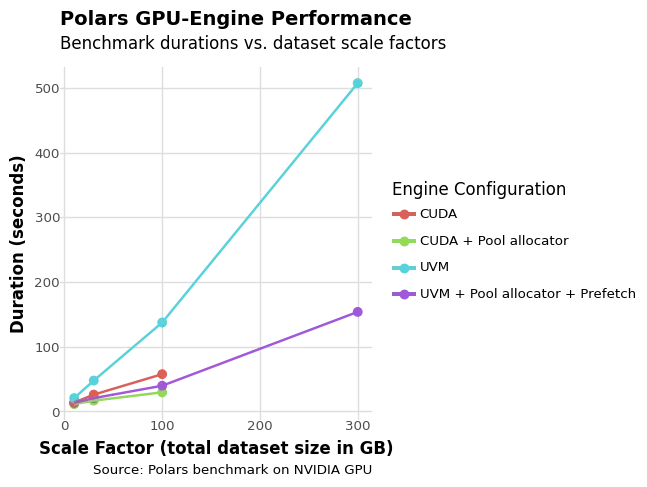 Figure 1. Benchmark results with different GPU Engine configurations on different dataset scales.
From this figure we can observe several key performance patterns that reveal the complex tradeoffs between different memory management approaches:
- Notably, while UVM successfully processes all queries in the 300GB dataset without running out of memory, the CUDA + Pool configuration fails on the first query despite handling nearly all other queries successfully with only 141GB of VRAM available. This pattern highlights how query execution success depends heavily on the specific memory access patterns and requirements of individual scenarios rather than just overall memory capacity.
- The pool sub-allocator consistently demonstrates its value as an optimization layer, reducing benchmark runtime by 15% on smaller datasets (scale factor 10) and up to 60% on larger datasets (scale factor 300), making it an easy default choice for most configurations.
- As expected, the base UVM configuration shows significant performance penalties, running 1.5x to 2.4x slower than the base CUDA configuration due to the absence of intelligent page migration mechanisms. In this worst-case scenario, every memory access that isn’t already in VRAM triggers a page fault, causing severe memory performance degradation as items are swapped into VRAM on demand.
- However, when UVM incorporates both pool allocation and prefetching, this performance penalty shrinks considerably to just 1.2x to 1.3x slower than CUDA, demonstrating the effectiveness of proactive memory management.
Additionally, we can conclude that UVM allows for executing queries above the memory threshold that a configuration without UVM could process. This happens at a slight cost of performance, however. This also means that in some cases, despite your dataset being too large to fit into VRAM in its entirety, you might be able to still process it without UVM.
Your Mileage May Vary
Ultimately what you should pick will depend on your use case. The big factors are the hardware that is available to you, the data you’re working with, and what your query looks like. Luckily trying out these engine configurations is as easy as adapting only the .collect(...) call. Be sure to benchmark a couple of times (using tools like hyperfine, py-spy, or Scalene) and pick the one that suits you best!