Polars in Aggregate: Polars Cloud, Streaming engine, and New Data Types

Since the last edition of Polars in Aggregate one year ago:

• 37 releases have been published.
• 2323 PRs were merged.
• 175474 lines of code were removed.
• 316565 lines of code were added.

This post summarizes the biggest highlights of that work.

Polars Cloud is Live

Whether you are processing a few hundred rows or billions of records, the syntax and development workflow remains the same. You should be able to write code once and run it anywhere, bringing a Unified API for data at every scale. This is exactly what our new distributed engine enables. On top of that, we handle the infrastructure for your query by automatically spinning up and tearing down compute resources on your own account, ensuring data never leaves your environment.

Get started on Polars Cloud in 10 minutes: https://docs.pola.rs/polars-cloud/quickstart/

Highlighted Features

On a more technical note, here’s an overview of the most important new features:

Next-Generation Streaming Engine

PR: #20947

Experimenting with our previous streaming engine taught us everything we needed to know to do it right. Based on research like Morsel-Driven Parallelism we’ve optimized this engine for performance and scalability.

The figure below is taken from the benchmark in May where we ran the PDS-H benchmark on our engines. You can see the difference in performance:

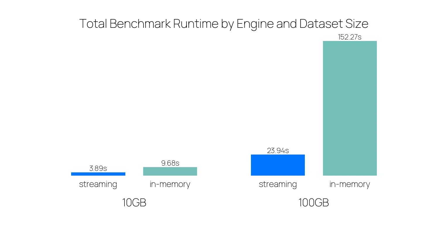
As the dataset size increases, the performance of the streaming engine improves significantly compared to the in-memory engine.

You can use this engine in a couple of ways:

• lf.sink_*(): the lazy, memory-efficient alternative to df.write_*() that streams your data directly to a file, allowing you to write results directly to disk without collecting results to a DataFrame first. The results can often be written in a streaming fashion. This method runs the query on the streaming engine by default.
• pl.Config.set_engine_affinity("streaming"): set an engine affinity from that point on, running everything on the streaming engine. It should be put at the beginning of your code.
• lf.collect(engine="streaming"): collect LazyFrames in streaming mode explicitly.

We already recommend using the streaming engine. In case a part of the query is not supported by the streaming engine, it will silently fall back to the in-memory engine for just the parts that aren’t supported. We’ll soon set the streaming engine as the default engine for processing your queries.

The Categorical Overhaul

PR: #23016

The introduction of the new streaming engine taught us that the old Categorical design was no longer sufficient and needed an overhaul. To make them work we no longer use the scoped or global StringCache. Users can now specify a Categories object that defines the scope.

Categories contain a name, namespace, and an underlying physical type. The name is used to identify the category, can be left empty to create or refer to a global category. If you have categories that share the same name but represent different things, you can use the namespace to distinguish them and prevent collisions. Lastly, you can specify the underlying physical type for memory optimization, which can be UInt8 (encodes up to 255 categories), UInt16 (up to 65535 categories), or, the default: UInt32 (up to 4294967295 categories). Two Categories are considered the same if all of these three parameters match.

df = pl.DataFrame({"animal": ["cat", "dog", "bunny", "dog"]}).cast(pl.Categorical())
df

shape: (4, 1)
┌────────┐
│ animal │
│ ---    │
│ cat    │
╞════════╡
│ cat    │
│ dog    │
│ bunny  │
│ dog    │
└────────┘

Categories can be retrieved from a Categorical by getting the categories attribute of a Categorical dtype. It will behave like a Python dictionary that works bidirectionally, like so:

categories = df.get_column("animal").dtype.categories
print(categories[1])  # Physical type
print(categories["dog"])  # Category

'dog'
1

Enums are a specialized type of Categories that are frozen and have a fixed set of categories that you provide up front. They are useful for efficiently representing a set of known values, such as days of the week, colors, or products. The order of the categories can be determined by the order in which they are provided:

priority = pl.Enum(["High", "Medium", "Low"])

s = pl.Series("tasks", ["High", "Low", "Medium", "High", "Low"], dtype=priority)

s.sort()

shape: (5,)
Series: 'tasks' [enum]
[
	"High"
	"High"
	"Medium"
	"Low"
	"Low"
]

If you already know the categories of a column, the Enum is the preferred way to define them.

Decimal is Stable, and Introducing Int128

PRs: #25020 (Stabilize decimal), #20232 (Int128Type)

Speed is only useful if the answer is correct. Standard floating-point arithmetic (0.1 + 0.2) results in 0.30000000000000004, which can be a dealbreaker in scientific and financial sectors. On top of that, floats are non-associative, meaning the order of operations changes the result. Because of precision loss when mixing scales, such as the classic (Big + -Big) + Small case, grouping, (a + b) + c can yield a different value than a + (b + c):

df = pl.DataFrame({"a": [1e16], "b": [-1e16], "c": [1.0]})

df.select(
    result_1 = (pl.col("a") + pl.col("b")) + pl.col("c"),
    result_2 = pl.col("a") + (pl.col("b") + pl.col("c")),
)

shape: (1, 2)
┌──────────┬──────────┐
│ result_1 ┆ result_2 │
│ ---      ┆ ---      │
│ f64      ┆ f64      │
╞══════════╪══════════╡
│ 1.0      ┆ 0.0      │
└──────────┴──────────┘

We are happy to announce that the Decimal type is now stable, which resolves this.

Decimals work with two parameters, precision and scale. precision is the total number of digits in a number, while scale is the number of digits to the right of the decimal point.

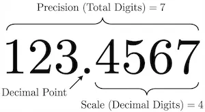
Decimal uses 128 bits which allows for a maximum precision of 38 digits. The scale can be set anywhere from 0 to the precision, depending on your data, and remains fixed over calculations. We round accordingly to retain the set scale. We deliberately chose this fixed-scale design over the traditional SQL approach where scales expand during operations (e.g., where multiplication results in scale_1 + scale_2).

In traditional systems, multiplying two columns with a scale of 20 would result in a scale of 40, immediately overflowing the 38-digit limit of 128-bit decimals. By enforcing a fixed scale, we avoid these ‘exploding scale’ issues and provide the behavior most users actually expect: if you are calculating currency with 2 decimal places, you usually want the result to remain at 2 decimal places without having to manually cast the type at every step.

For example:

import polars as pl
from decimal import Decimal

df = pl.DataFrame(
    {
        "amount": [Decimal("123.4567"), Decimal("123.45"), Decimal("123.456789")]
    }, 
    schema={"amount": pl.Decimal(precision=7, scale=4)},
)
df

shape: (3, 1)
┌──────────────┐
│ amount       │
│ ---          │
│ decimal[7,4] │
╞══════════════╡
│ 123.4567     │
│ 123.4500     │
│ 123.4568     │
└──────────────┘

In this example, you can see that less precise decimals get padded with zeroes, and more precise decimals get rounded according to precision.

Besides the Decimal, we’re also introducing the new Int128 type, allowing for massive integer ranges. Compared to the previous biggest int, Int64, it uses double the memory space and, thanks to exponential scaling, captures a range roughly 18 quintillion times larger. This allows you to work with integers ranging from -1.7e+38 to 1.7e+38, (which is 2^127).

Create a Generator with lf.collect_batches()

PR: #23980

While lf.sink_parquet() and other native sinks are the fastest way to write data, sometimes you want to process output data yourself.

Previously, this required either collecting the whole result into RAM with lf.collect() (risking an OOM error) or manually slicing the LazyFrame (which is tedious and slow). The new lf.collect_batches() method solves this by yielding a Python generator of sub-DataFrames instead of one final result.

This allows you to “peel off” chunks of processed data, handle them in Python, and discard them to free up memory before the next chunk arrives.

# The engine pauses and yields control to Python every ~50k rows
for i, batch_df in enumerate(large_lf.collect_batches(chunk_size=50_000)):
    custom_batch_logic(batch_df)

Because this method involves passing data back and forth between the Rust engine and Python, it will always be slower than a native sink. It is best used only when you need to implement custom logic that cannot be handled by standard sinks.

Improvements

Besides these features, several other enhancements have been introduced:

Common Subplan Elimination in collect_all

PR: #21747

When you have multiple LazyFrames derived from the same source data, treating them individually can be inefficient when several queries share some common transformations of the source.

If you run df1.collect() and df2.collect() separately, Polars might read the source file twice or compute the same operation multiple times. We have introduced Common Subplan Elimination (CSE) into pl.collect_all(). When you pass a list of LazyFrames to collect_all(), the optimizer now analyzes the entire graph of all frames combined. It identifies shared branches (like a common scan_parquet and filter operation) and executes them once, caching the result for both downstream outputs. This can result in big performance improvements by doing work only once.

import polars as pl
import time

# Generate expensive LazyFrame with 10M rows
base = pl.LazyFrame({
    "customer_id": pl.int_range(0, 10_000, eager=True).sample(n=10_000_000, with_replacement=True),
    "product_id": pl.int_range(0, 500, eager=True).sample(n=10_000_000, with_replacement=True),
    "amount": pl.int_range(10, 1000, eager=True).sample(n=10_000_000, with_replacement=True),
}).filter(pl.col("amount") > 100)

# Three queries from same base
q1 = base.group_by("customer_id").agg(pl.col("amount").sum())
q2 = base.group_by("product_id").agg(pl.col("amount").mean())
q3 = base.filter(pl.col("amount") > 500).select(pl.col("amount").max())

# Without CSE: processes base 3 times
start = time.time()
r1, r2, r3 = q1.collect(), q2.collect(), q3.collect()
print(f"Without CSE: {time.time() - start:.2f}s")

# With CSE: processes base once
start = time.time()
r1, r2, r3 = pl.collect_all([q1, q2, q3])
print(f"With CSE: {time.time() - start:.2f}s")

Without CSE: 1.58s
With CSE: 1.01s

In this toy example it leads to a ~35% performance increase, but your mileage may vary depending on your use case.

Another example of what is now possible is if you only want to create a file when it also passes a validation in streaming fashion. You can multiplex that:

lf = expensive_operation()

q1 = lf.map_batches(lambda x: validate(x)) # Throws ValidationError when invalid
q2 = lf.sink_parquet("output.parquet", lazy=True)

try:
    pl.collect_all([q1, q2])
except ValidationError:
    os.remove("output.parquet")

Introducing Polars Runtimes

PR: #24531 (Ordering), #25284 (Runtime refactor)

You might’ve already noticed that on new installations besides polars a library named polars-runtime-32 is also installed. Polars now has different runtimes in which features and optimizations are exposed for different system configurations.

Historically, it was not possible to have packages depend on different Polars runtimes as they were built into different PyPI packages (e.g. polars-lts-cpu, polars-u64-index). Importing Polars could load any of those packages in an unpredictable manner, which could lead to strange shadowing issues.

With the introduction of the runtimes, this will be resolved by Polars automatically and deterministically. Polars will load the most conservative runtime that is available on your system.

Alternative runtimes can now be downloaded by setting the correct extras when installing Polars, for example: uv pip install "polars[rtcompat]".

The runtime loading hierarchy is now:

Loading priority	Pip install name	Runtime name	Formerly known as
1.	polars[rtcompat]	polars-runtime-compat	polars-lts-cpu
2.	polars[rt64]	polars-runtime-64	polars-u64-index
3.	polars	polars-runtime-32	polars

And Much More

This is just a glimpse of what we’ve built. If you want to stay up to date, you can follow us on the following social platforms:

[LinkedIn] - [Twitter/X] - [Bluesky]

Or you can learn more about Polars Cloud at: https://cloud.pola.rs/