Announcing Polars 1.43

Polars 1.43 is out. This release brings two new expressions, two faster joins, and a linear-time rolling aggregation: nested lists from multiple columns, exponentially weighted sums, joins that only scan the partitions they need, a hint for which side a join uses as its build side, and rolling min_by/max_by that no longer recompute each window from scratch.

Pack columns into nested lists with pl.list()

Each column’s value stays intact as its own element, instead of merging into one flat list.

PR: #27990

Sometimes you want to pack a row’s values into a list while keeping each column’s value intact as its own element, for example building a list[list[...]] where downstream code processes one column’s contribution at a time. concat_list can’t express this: it flattens List-typed inputs into one level instead of nesting them.

Polars already had concat_list for combining columns into a List. Run it on two List-typed columns and pl.list() side by side on the same data:

import polars as pl

df = pl.DataFrame({"a": [[1, 2], [3], [4, 5]], "b": [[6], [7, 8], [9]]})

df.with_columns(a_b=pl.concat_list("a", "b"))
# Output
# shape: (3, 3)
# ┌───────────┬───────────┬───────────┐
# │ a         ┆ b         ┆ a_b       │
# │ ---       ┆ ---       ┆ ---       │
# │ list[i64] ┆ list[i64] ┆ list[i64] │
# ╞═══════════╪═══════════╪═══════════╡
# │ [1, 2]    ┆ [6]       ┆ [1, 2, 6] │
# │ [3]       ┆ [7, 8]    ┆ [3, 7, 8] │
# │ [4, 5]    ┆ [9]       ┆ [4, 5, 9] │
# └───────────┴───────────┴───────────┘

df.with_columns(a_b=pl.list("a", "b"))
# Output
# shape: (3, 3)
# ┌───────────┬───────────┬─────────────────┐
# │ a         ┆ b         ┆ a_b             │
# │ ---       ┆ ---       ┆ ---             │
# │ list[i64] ┆ list[i64] ┆ list[list[i64]] │
# ╞═══════════╪═══════════╪═════════════════╡
# │ [1, 2]    ┆ [6]       ┆ [[1, 2], [6]]   │
# │ [3]       ┆ [7, 8]    ┆ [[3], [7, 8]]   │
# │ [4, 5]    ┆ [9]       ┆ [[4, 5], [9]]   │
# └───────────┴───────────┴─────────────────┘

concat_list flattens the two List columns into one. pl.list() keeps each row’s value from a and b intact as its own element, so a_b ends up as list[list[i64]] instead of list[i64].

On scalar columns the two are equivalent, since there is no nesting to flatten:

import polars as pl

df = pl.DataFrame({"a": [1, 2, 3], "b": [4, 5, 6]})
df.with_columns(a_b=pl.list("a", "b"))

# Output
# shape: (3, 3)
# ┌─────┬─────┬───────────┐
# │ a   ┆ b   ┆ a_b       │
# │ --- ┆ --- ┆ ---       │
# │ i64 ┆ i64 ┆ list[i64] │
# ╞═════╪═════╪═══════════╡
# │ 1   ┆ 4   ┆ [1, 4]    │
# │ 2   ┆ 5   ┆ [2, 5]    │
# │ 3   ┆ 6   ┆ [3, 6]    │
# └─────┴─────┴───────────┘

Exponentially weighted sums with ewm_sum

A running total where recent values count more than old ones, instead of a plain cumulative sum.

PR: #28215

Polars already had ewm_mean and ewm_mean_by for exponentially weighted moving averages, which normalize by the decayed weights so the result stays on the same scale as the input. 1.43 adds the summed counterparts, ewm_sum and ewm_sum_by, which skip that normalization and accumulate instead. That makes them a fit for decaying totals like cumulative volume or exposure, where you want older activity to fade out rather than average away.

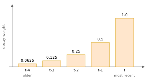
ewm_sum computes a decay-weighted running total over row order. With decay factor λ = 1 - α, it follows the same recurrence as ewm_mean: y₀ = x₀, and yᵢ = xᵢ + λ · yᵢ₋₁ for i > 0. Specify the decay with exactly one of com, span, half_life, or alpha.

import polars as pl

df = pl.DataFrame({"a": [1, 2, 3]})
df.with_columns(ewm_sum=pl.col("a").ewm_sum(alpha=0.5))

# Output
# shape: (3, 2)
# ┌─────┬─────────┐
# │ a   ┆ ewm_sum │
# │ --- ┆ ---     │
# │ i64 ┆ f64     │
# ╞═════╪═════════╡
# │ 1   ┆ 1.0     │
# │ 2   ┆ 2.5     │
# │ 3   ┆ 4.25    │
# └─────┴─────────┘

ewm_sum_by weights the decay by the spacing between values in a by column instead of by row position, mirroring ewm_mean_by. The decay factor for each step becomes λᵢ = exp(-ln(2) · (tᵢ - tᵢ₋₁) / τ), where τ is half_life, so a bigger gap between two observations decays the running total more than a small one does.

df = pl.DataFrame({
    "values": [1, 2, 3, 4, 5],
    "times": [0, 1, 2, 5, 6],
})
df.with_columns(ewm_sum=pl.col("values").ewm_sum_by("times", half_life="1i"))

# Output
# shape: (5, 3)
# ┌────────┬───────┬──────────┐
# │ values ┆ times ┆ ewm_sum  │
# │ ---    ┆ ---   ┆ ---      │
# │ i64    ┆ i64   ┆ f64      │
# ╞════════╪═══════╪══════════╡
# │ 1      ┆ 0     ┆ 1.0      │
# │ 2      ┆ 1     ┆ 2.5      │
# │ 3      ┆ 2     ┆ 4.25     │
# │ 4      ┆ 5     ┆ 4.53125  │
# │ 5      ┆ 6     ┆ 7.265625 │
# └────────┴───────┴──────────┘

The gap between index 2 and index 5 is larger than the other steps, so the running sum decays more there than it would with evenly spaced points. half_life also accepts calendar durations like "1d" or "2h" for a temporal by column, or a timedelta. Both ewm_sum and ewm_sum_by are marked unstable and may change without a breaking-change notice.

Steer which side a join builds

Override which frame Polars builds its hash table from, when you know better than the heuristic.

PR: #28154

Joining two DataFrames means matching rows between them on a key. Polars does this with a hash join, and it has to decide which of the two frames to build its hash table from: the build side. Polars already chooses automatically, favoring the frame with the fewest unique keys, but 1.43 adds a build_side argument to join() so you can bias or override that choice.

import polars as pl

big = pl.LazyFrame({"key": range(1_000_000), "v": range(1_000_000)})
small = pl.LazyFrame({"key": [1, 2, 3], "label": ["a", "b", "c"]})

result = (
    big.join(small, on="key", how="inner", build_side="force_right")
    .collect(engine="streaming")
)

# Output
# shape: (3, 3)
# ┌─────┬─────┬───────┐
# │ key ┆ v   ┆ label │
# │ --- ┆ --- ┆ ---   │
# │ i64 ┆ i64 ┆ str   │
# ╞═════╪═════╪═══════╡
# │ 3   ┆ 3   ┆ c     │
# │ 2   ┆ 2   ┆ b     │
# │ 1   ┆ 1   ┆ a     │
# └─────┴─────┴───────┘

build_side="force_right" guarantees the 3-row small frame becomes the build side, instead of the 1,000,000-row big frame.

build_side accepts five values:

• "auto": the default, unchanged automatic behavior.
• "prefer_left" / "prefer_right": bias the existing heuristic toward one side without overriding it outright.
• "force_left" / "force_right": pin the build side regardless of what the heuristic would pick.

This parameter is marked experimental and currently only affects the streaming engine. The old in-memory engine ignores it.

Faster joins on hive-partitioned data

Join only the partitions that can actually match, instead of scanning and joining everything.

PR: #28327, #28374

When both sides of a join scan hive-partitioned data, the optimizer now rewrites the join into a union of per-partition joins. Instead of loading the union of all partition paths on both sides and joining once, it loads only the partitions whose keys can match, and runs a separate join per matching partition pair. 1.43 covers inner joins (#28327), and extends the same rewrite to left, right, and semi joins (#28374).

For a join on foo=1/foo=2 hive partitions against bar=1/bar=2 partitions, show_graph(engine="streaming") makes the rewrite visible:

import polars as pl

left = pl.scan_parquet("parts1", hive_partitioning=True)
right = pl.scan_parquet("parts2", hive_partitioning=True)

left.join(
    right, left_on=["foo", "key"], right_on=["bar", "key"], how="inner"
).show_graph(engine="streaming")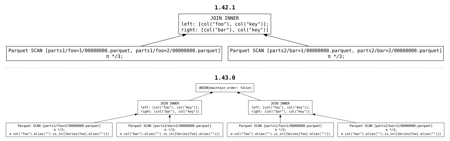

On 1.42.1, both sides are scanned in full and joined once. On 1.43.0, the plan is a UNION of two independent joins, one per matching partition pair, and each side only scans its own partition.

Only the partitions that can actually match are scanned, and each side of each join has a smaller build side, which helps memory use and cache hit rate. On the distributed engine, this also elides shuffles entirely: each partition pair is processed independently and in parallel. There is no API change, and the rewrite applies automatically to joins over scan_parquet/scan_csv/etc. with hive_partitioning=True.

Partitions	Rows per partition	Before	After	Speedup
16	1,000,000	0.370s	0.185s	2.00x

Benchmark: inner join of two hive-partitioned Parquet datasets sharing a partition key (16 partitions, 1,000,000 rows per partition per side, unique keys), median of 5 runs on an Apple M4 Pro, comparing uv run --with "polars==1.42.1" against uv run --with "polars==1.43.0". Every partition pair matches here, which is a best-case scenario for the rewrite. Datasets where most partition pairs cannot match at all will see larger gains from the pruning itself.

Rolling min_by / max_by in linear time

Rolling windows that pick their extremum by another column no longer recompute it from scratch every time.

PR: #27436

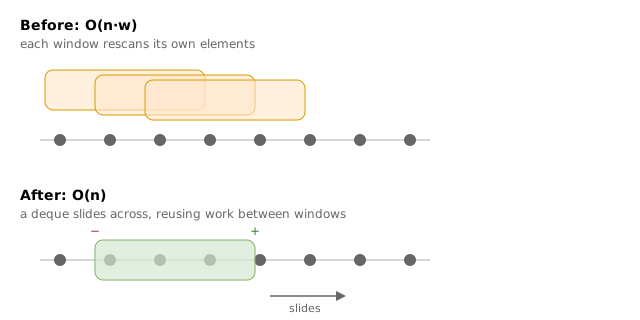
min_by and max_by return the value of one column at the position where another column is smallest or largest. Used inside DataFrame.rolling().agg(...), each window used to recompute its extremum independently, which is O(n·w) for window size w. 1.43 adds a monotonic-deque fast path that slides across overlapping windows in amortized O(n) instead:

import polars as pl
from datetime import datetime, timedelta

df = pl.DataFrame({
    "time": [datetime(2026, 1, 1) + timedelta(days=i) for i in range(6)],
    "value": [5, 3, 8, 1, 9, 4],
    "sensor": [30, 10, 50, 20, 60, 40],
})

df.rolling(index_column="time", period="3d").agg(
    pl.col("value").min_by("sensor").alias("min_val"),
    pl.col("value").max_by("sensor").alias("max_val"),
)

# Output
# shape: (6, 3)
# ┌─────────────────────┬─────────┬─────────┐
# │ time                ┆ min_val ┆ max_val │
# │ ---                 ┆ ---     ┆ ---     │
# │ datetime[μs]        ┆ i64     ┆ i64     │
# ╞═════════════════════╪═════════╪═════════╡
# │ 2026-01-01 00:00:00 ┆ 5       ┆ 5       │
# │ 2026-01-02 00:00:00 ┆ 3       ┆ 5       │
# │ 2026-01-03 00:00:00 ┆ 3       ┆ 8       │
# │ 2026-01-04 00:00:00 ┆ 3       ┆ 8       │
# │ 2026-01-05 00:00:00 ┆ 1       ┆ 9       │
# │ 2026-01-06 00:00:00 ┆ 1       ┆ 9       │
# └─────────────────────┴─────────┴─────────┘

sensor is independent of time, so the row with the smallest or largest sensor value shifts around as each window gains and drops rows, and min_val/max_val track it accordingly. The fast path activates when both the window groups and the by column’s groups are monotonic and overlapping, and the by column is numeric. Non-numeric by columns fall back to the existing algorithm. There is no API change.

Rows	Window size	Before	After	Speedup
2,000,000	~200,000	0.0163s	0.0128s	1.27x

Benchmark: rolling(index_column=...).agg(pl.col("value").min_by("sensor")) (and max_by), same shape as the example above but at scale. Median of 5 runs on an Apple M4 Pro, comparing uv run --with "polars==1.42.0" against uv run --with "polars==1.43.0". If sensor were the rolling index itself, the arg-min/arg-max position would always be the window’s first or last row and both versions would be equally fast regardless of window size.

And More

The full list of changes is in the 1.43 release notes on GitHub.

Follow us for updates:

[LinkedIn] - [Twitter/X] - [Bluesky] - [GitHub]