A new streaming backend for the Polars GPU engine

At NVIDIA we launched the Polars GPU engine together with the Polars team in 2024, built on an in-memory executor that ran a query on one GPU. Since then, the most consistent thing we have heard from users is that they want more headroom: larger datasets, and the ability to process with multiple GPUs. A first, experimental version of that shipped in 25.06 as a Dask-orchestrated streaming executor.

As of the 26.06 release of cudf-polars, the Polars GPU engine runs on a new streaming backend built on RapidsMPF, a library for streaming and multi-GPU execution. It is a substantially faster rewrite of that earlier executor and is now the recommended path for any nontrivial GPU workload.

The streaming executor partitions data into chunks and flows them through the query graph, with RapidsMPF managing the data movement underneath. Two capabilities follow from that:

• Queries are no longer bound by GPU memory. Chunks spill to host memory when device memory gets tight, so a single GPU can work through datasets many times its own capacity.
• The same query scales from one GPU to many. Multi-GPU execution runs the same executor across more GPUs rather than a separate code path.

The CPU engine is highly optimized for interactive and medium-scale analytics on a single node, and for a great deal of work it remains the right tool. As datasets grow into the hundreds of gigabytes and beyond, however, the expensive parts of a query (joins, high-cardinality group-bys, sorts) can slow down drastically, and those are the operations the GPU engine accelerates most.

The sections below cover how to run this new engine, how the backend works, and how it can be used to accelerate TB-scale benchmarks by up to 23x.

Setup

The engine ships as the cudf-polars package. Follow the installation guide and pick the build matching your CUDA and Python versions:

# pip, CUDA 12 by default
pip install "polars[gpu]"
# for CUDA 13
pip install cudf-polars-cu13

# or conda
conda install -c rapidsai -c conda-forge cudf-polars

You select GPU execution by passing an engine= argument to .collect() calls. The simplest form is setting engine to "gpu", which runs the query on a single GPU with no additional setup:

import polars as pl

query = (
    pl.scan_parquet("/data/dataset/*.parquet")
    .group_by("customer_id")
    .agg(pl.col("amount").sum())
)

result = query.collect(engine="gpu")

To use more than one GPU, or to tune the engine’s configuration, construct an engine object instead. The examples in this post use RayEngine, but DaskEngine and SPMDEngine are equally supported, and the engines documentation covers when you might prefer each. Each has a corresponding pip extra:

pip install "cudf-polars-cu13[ray]"  # or dask

Constructed with no arguments, RayEngine uses every GPU visible to the process:

from cudf_polars.engine.ray import RayEngine

with RayEngine() as engine:
    result = query.collect(engine=engine)

That is the complete setup for single-node multi-GPU execution. There is no cluster to configure, no partitioning scheme to specify, and no change to the query itself. Tuning knobs such as chunk size, spilling behavior, and fallback mode are set through a StreamingOptions object that every streaming engine accepts. See the configuration options reference for the full list.

The layer above the engine is unchanged Polars. You write the same LazyFrame, and the Polars optimizer runs before the plan reaches cudf-polars. We hook in after the optimized IR is built, so semantics, type inference, and optimizations match what you would get on the CPU. Operations the GPU engine does not support fall back to the CPU engine by default.

How RapidsMPF makes this work

RapidsMPF contributes two things to the GPU engine: a streaming execution framework, and a set of communication primitives optimized for moving data between GPUs. Together they allow a query to exceed both the memory and the compute of a single GPU.

Streaming execution and out-of-core processing

The engine decomposes inputs into chunks and flows them through the query graph, filtering, transforming, aggregating, and joining chunk by chunk. Chunk size is chosen to leave headroom for the intermediate buffers each operation needs, since the executor overlaps many operations concurrently.

The execution framework itself is modeled on Hoare’s Communicating Sequential Processes. Each physical operation in the query plan becomes a long-lived actor coroutine, and actors are connected by bounded-capacity channels: a scan feeds a select feeds a filter feeds a sink. Bounded channels provide backpressure, so a slow consumer throttles its producer rather than accumulating an unbounded queue in GPU memory. This keeps memory use predictable even with many operations in flight.

This is where the two capabilities above come from. Chunks that are not actively being processed spill to host memory under memory pressure and are pulled back when needed, which is what lets a single GPU work through a dataset many times the size of its VRAM. The same decomposition then carries over to multiple GPUs: the chunking that lets one GPU stream through a 1 TB dataset is what lets eight split it.

This is the execution model for every way of running the engine. RayEngine, DaskEngine, and SPMDEngine all drive the same streaming executor and differ only in how GPU workers get provisioned, so the choice is about how you prefer to deploy rather than about performance.

Optimized communication primitives

Scaling a dataframe engine across GPUs is largely a data movement problem. Joins, sorts, and high-cardinality group-bys all need rows with matching keys to end up on the same GPU, which requires an all-to-all shuffle. Shuffles are a common failure point for distributed query engines, since every participating process, one per GPU and referred to as a rank, must hold both the data it is sending and the data it is receiving.

RapidsMPF implements the shuffle as a streaming collective. Each rank inserts chunks of a partitioned table as they are produced, and RapidsMPF routes each chunk to the rank that owns its hash key as soon as it arrives, so data crosses the network while the operators feeding the shuffle are still producing more. Once every rank has finished inserting, each rank extracts the chunks it now owns. Other collectives such as AllGather follow the same pattern.

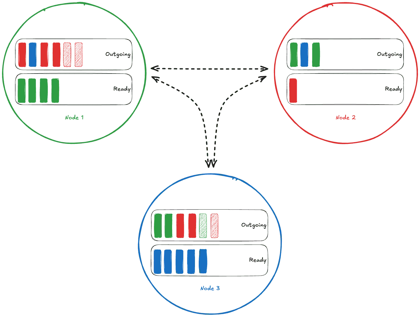
Because the size of a rank’s output is not knowable until all input has been seen, RapidsMPF allocates those output buffers itself. That also lets it spill them: under memory pressure, chunks move to host memory and return when the operation that needs them resumes. This is what allows a shuffle to complete when the data involved exceeds device memory.

Underneath the collectives sits a communicator abstraction implemented over UCX/UCXX or MPI, which handles CPU and GPU data uniformly and lets the transport select the appropriate route between any two ranks. Scaling from one GPU to multiple is therefore a change in rank count rather than in program structure.

For the full mechanics, the RapidsMPF background docs cover the shuffle architecture, channels, and actor model in detail.

Benchmarks

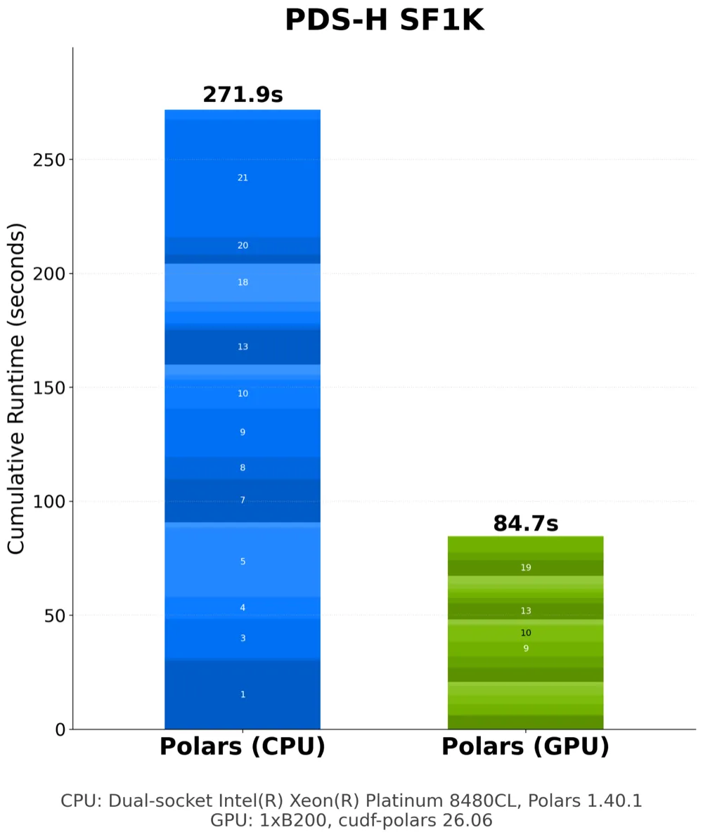
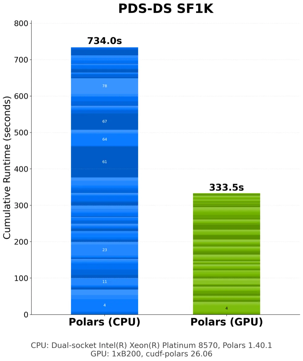
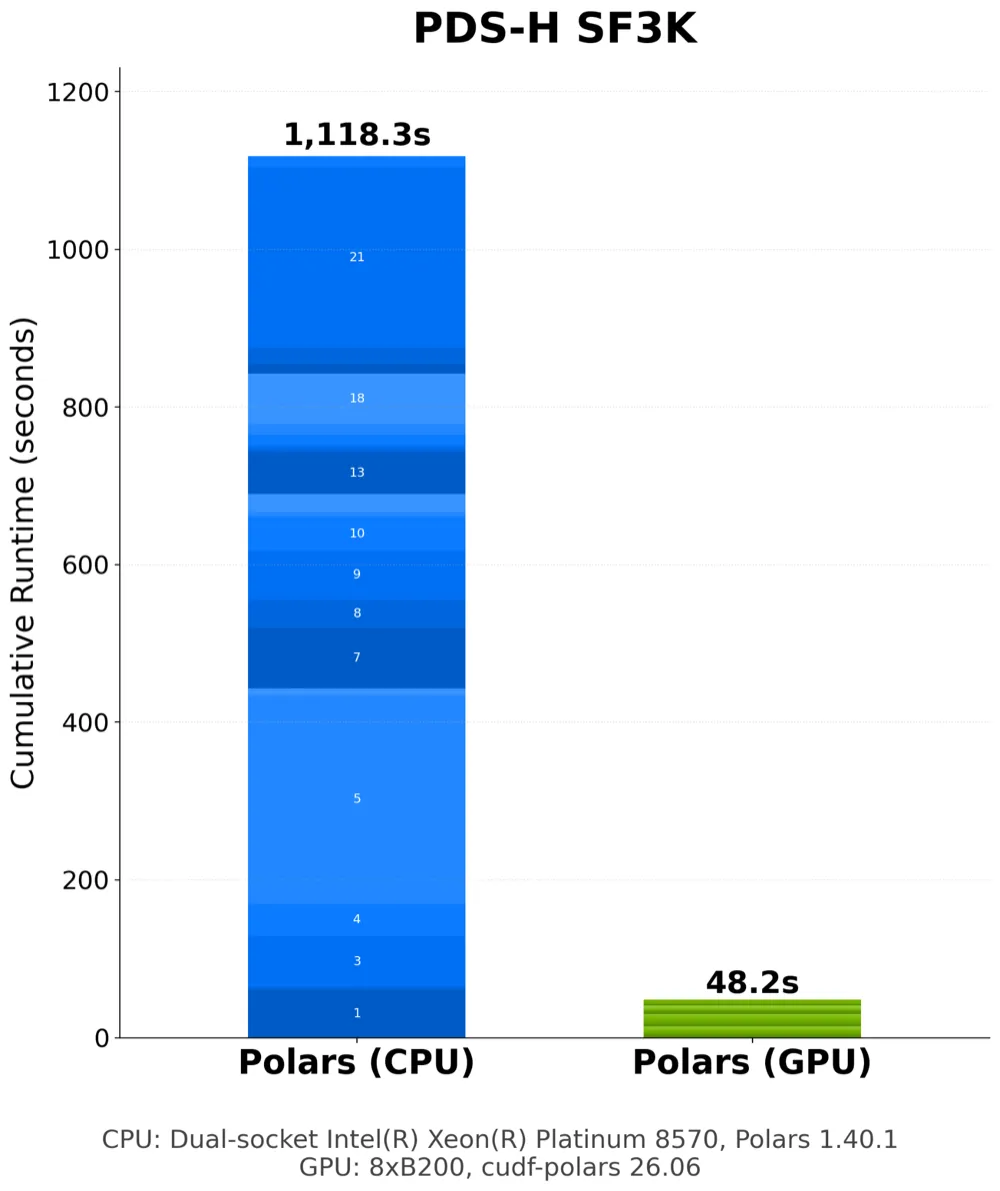
To show what this looks like at scale, we ran PDS-H and PDS-DS at terabyte scale.¹

At SF1K, roughly 1 TB of uncompressed data, a single GPU runs the full PDS-H suite 3.2x faster than the CPU engine and PDS-DS 2.2x faster:

At SF3K, roughly 3 TB, scaling out across eight GPUs widens that to 23.2x on PDS-H and 11.0x on PDS-DS:

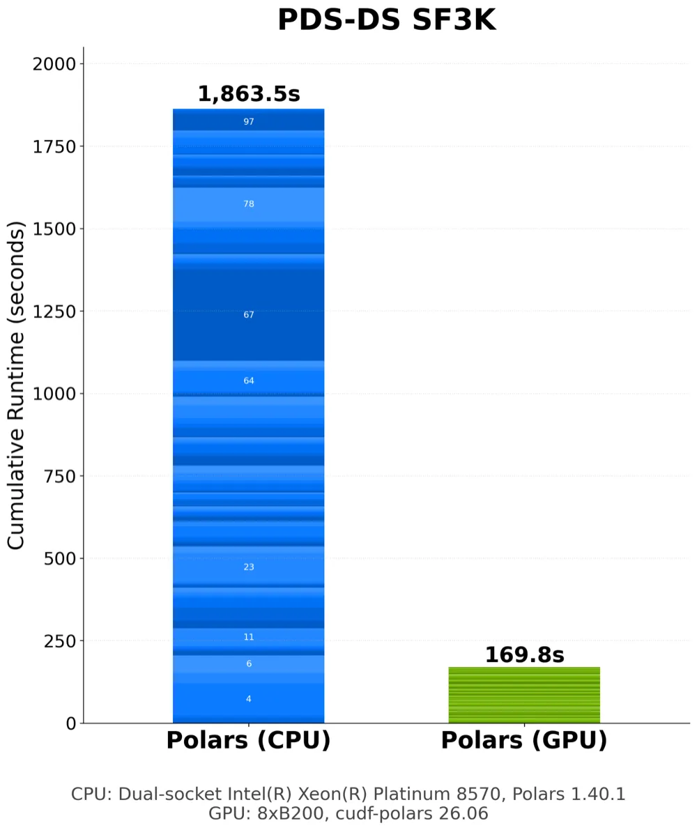
The benchmarks are reproducible end to end. The benchmark docs walk PDS-H through data generation with tpchgen-cli, along with the CPU, single-GPU, and multi-GPU runner invocations. The query implementations for both suites live in the cuDF repository.

Try it on your own data

If you have a Polars pipeline whose runtime makes iteration difficult, the GPU engine is straightforward to evaluate. Install cudf-polars and add engine="gpu" to an existing .collect() to get a baseline on one GPU. From there, RayEngine spreads the same query across every available GPU. Unsupported operations fall back to the CPU engine, so an existing query can be run as-is.

The Polars GPU support guide documents current limitations, and the cudf-polars documentation covers engines, configuration, and memory tuning in depth.

The engine is under active development, and feedback is welcome. Feature requests and API coverage gaps are best filed on the cuDF repository, and you can also find us in the Polars Discord.

Footnotes

1. Polars Decision Support (PDS-H and PDS-DS) are open implementations derived from the TPC-H and TPC-DS benchmarks. They use the TPC data models, data generation methodology, and query workloads to measure analytical query performance across a range of dataset sizes. While they closely follow the TPC specifications, they are not officially audited or certified TPC benchmarks. Consequently, PDS results are intended for comparative evaluation within PDS and are not directly comparable to published TPC benchmark results. ↩