Preface
Recently, METRO.digital initiated a project to enhance the creation of Key Performance Indicators (KPIs) across 19 countries for METRO. By migrating from SQL to Python and leveraging Polars, they achieved significant improvements in efficiency, readability and maintainability.
In this case study Dr. Patrick Bormann (Tech lead data scientist) shares his team’s experiences.
About METRO.Digital
METRO.digital is the tech product-led company of METRO, the leading international specialist for wholesale and food trade. METRO operates in more than 30 countries worldwide and has products in over 623 wholesale stores and 94 delivery depots, as well as the online marketplace METRO MARKETS.
With longstanding experience in global wholesale, METRO.digital develops customized IT services and products worldwide for all METRO countries. Located in Germany, Romania and Vietnam, the METRO.digital employees are working continuously on one goal: digitalizing the wholesale industry.
About the Project
Our team specializes in data science and specifically causal inference in machine learning, focusing on what-if scenarios, and using business and product KPIs to leverage our causal recommender systems. We aim to support decisions for category managers in the wholesale business by accelerating their decision making and offering better insights in strategic assortment reductions as humans might not notice all the details in complex decision-making systems. Our most recent project involved transforming SQL- based KPI creation into a Python-based process using Polars.
Main Goal: Improving Maintainability, Readability, and Preparing for Future KPI Enhancements
Our task was to convert 50 SQL files per KPI into Python code, while keeping the original KPI logic for 19 countries across the globe, having most of these countries in Europe.
One of our main acceptance criteria dictated that loading invoice data into memory must be fast and preprocessing even faster, so that changes on the KPI for future enhancements, while developing, were immediately visible, when working in a notebook environment.
We needed this immediate feedback, as we were not sure which parts of the code we could keep, which parts to enhance, and which parts may be even wrong as the code was not ours but inherited. However, speed was not the only key factor here, as you do not have a good grasp of what is going in your code with so many files for just one KPI. Although we knew that the amount and naming of the files followed a specific data warehouse structure, higher readability and easier maintenance in this case are absent. Yet, for us these aspects were as essential as speed in loading and preprocessing of data.
To get an idea with how much data we dealt with: One of our biggest countries has over 930 million rows and several columns of data for two years. Loading of data with schema overrides took only 8 minutes and preprocessing the data ran within mere seconds.
Having a Good Prior
Although we already decided to bring our 50 SQL files per KPI to Python, to make KPI creation more readable and maintainable, the question was of course, which tool to use. True there may have been other alternatives, like PySpark. Yet, we had previous experience, so to speak a good prior, with Polars in our causal recommender project. Yet, this experience was limited to the standard Polars library. Before, we only worked with a few million rows of data and not with data frames containing 180, 460 or even 930 million rows of invoice data as a maximum (as you will later see). We were quite sure that join operations on this scale could be quite challenging. Finally, we decided to give it a try and went for the polars-u64-idx library 1, and experimented with it.
Top-Down Readability
By migrating to Polars, we hoped to get a clear and structured way of creating our data. And indeed, it was easier to read Polars top down, instead of jumping within one SQL file. To get an idea, how a typical query looked like, consider both code snippets below:
CREATE OR REPLACE TABLE `${p_number}.${dt_ident}.product_dimensions`
AS
SELECT
    v.article_number,
    v.variant_number,
    v.article_brand_name,
    v.date_of_deletion,
    ph.stratified_id,
    (v.customer_number * 1000000000) + (v.article_number * 1000) + v.variant_number AS p_ATT_key,
    1 AS adjacent_sales,
CASE
    WHEN a.own_article > 0 THEN 1 ELSE 0
END AS is_own_article,
    (a.cat_level_one * 100) + a.cat_level_two AS grp_number
FROM `our-company-${country}-production_level.datawarehouse.variation` AS v
INNER JOIN `our-company-${country}-production_level.datawarehouse.articles` AS a
USING (customer_number, article_number)
LEFT JOIN `${p_number}.${dt_ident}.blocking_codes` AS pabcd
USING (article_number, variant_number)
LEFT JOIN `${p_number}.${dt_ident}.product_levels` AS pl
USING (article_number)
WHERE v.article_number > 0
    AND COALESCE(pabcd.block_code, 0) < 5
    AND pl.stratified_id NOT IN (60, 61)
And when using Polars:
product_dimensions = (
    variation
    .join(articles, on=["customer_number", "article_number"], how="inner", suffix="_a")
    .join(blocking_codes, on=["article_number", "variant_number"], how="left", suffix="_pabcd")
    .join(product_levels, on="article_number", how="left", suffix="_pl")
    .filter((pl.coalesce(['block_code', 0]) < 5) & (~pl.col('stratified_id').is_in([60, 61])))
    .with_columns(
        ((pl.col("customer_number")) + (pl.col('article_number') * 1000) + (pl.col('variant_number'))).alias("p_ATT_key"),
    )
    .select(
        'article_number',
        'variant_number',
        'article_brand_name',
        'stratified_id',
        'p_ATT_key',
        'grp_number'
    )
)
While some may argue that SQL appears more structured or easily to read, you can see that the migration revealed unnecessary filters, variables and bloated customer range numbers, which again put more burden on the KPI creation process.
Although cost reduction was not our primary goal, we appreciated the efficiency gains by removing these unnecessary computations.
Testing Piping of Lazy Plans
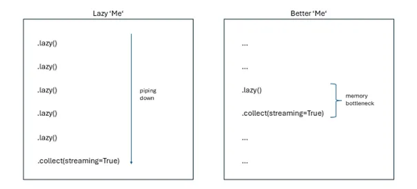
During our migration to Polars, we tested the piping of several lazy frames using the streaming engine, hoping that the optimized plans would reduce compute resources at the expense of longer calculation times for KPIs.
Using this approach blindly led to crashes and even increased compute resource usage. Additionally, piping multiple plans caused confusion due to so many unnamed sub plans crunched together in a final big plan. But was it the developers intention that it could be used for this? Maybe we did something wrong here. Maybe we should have used a graph to better explain all the piped plans. We remembered that in a precheck, we already limited the needed columns in the KPI creation process, maybe this limited the optimization in the first instance? In the end, selective usage was far more efficient, as the next paragraph shows.
Optimizing Joins with LazyFrames
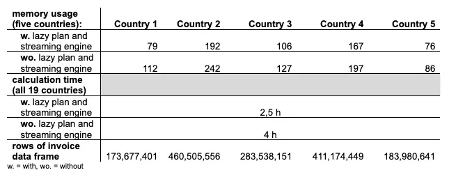
Instead of brute forcing plans into the pipe, we identified specific bottlenecks in the code, where joins of dataframes with billions of rows could benefit from lazy frames and the streaming engine. This optimization reduced compute resource requirements by 128GB of memory and 16 vCPUs, allowing for the use of a smaller machine type.
The following graphic shows the total amount of memory reduction for a few other countries. While the table does not tell 100% of the story, since some countries are missing in the calculation, we assume the larger the invoice data to be processed in the lazy plan, the more savings you gain in terms of compute resources 2.
So instead of being lazy ourselves, we decided to invest time in the question where the streaming engine would make sense:
Automated Shrinkage of Dtypes
We experimented also with automated shrinkage of dtypes with Polars internal
method of shrink_dtype. While shrinkage can be messy, especially for keys to be
joined on, selecting the larger union dtype for keys across several data frames made
it work. Yet, shrinkage led to wrong aggregations in Polars 1.5.0, which lead to the
decision to skip the shrinkage for columns, which would be needed in calculations.
However, it proved to be useful for columns that were sidekicks in the calculation
rather than main components. In 1.26.0 (latest version at time of writing) however, we encountered no problems at all.
assortment_levels = (
    df_info_numbers
    .with_columns(pl.col("company_id").cast(parent["parent_id"].dtype))
    .join(parent, left_on="company_id", right_on="parent_id", how="inner")
    .filter(
        (pl.col('date_from') <= date.today()) & (pl.col('date_to') >= date.today())
    )
    .pipe(shrink_dtypes)
    .with_columns(
        pl.col("article_number", "grp_number").cast(invoice["article_number"].dtype),
    )
)
To sum up, shrinkage helped us, to reduce RAM resources even more during the preprocessing of the KPIs. We encountered a reduction in occupied memory size by 50%, which can be a lot, especially for big data frames. Overall, lazy operations and shrinkage were the major contributors in reducing needed resources.
Conclusion
Migrating from SQL to Python using Polars brought significant benefits in readability, maintainability, and cost reduction, paving the way for future enhancements of our KPIs. Our project demonstrated clear advantages in using Polars for KPI creation, and we are excited to continue leveraging this state-of-the-art framework in future projects.